
Featured Post

Excel SUMIF Function Explained with Real Examples

If you work with numbers in Excel, there's one function you must master: SUMIF. It’s simple, powerful, and one of the most searched formulas globally. Whether you’re managing sales data, budgets, or reports, SUMIF helps you add values based on conditions — no filters needed. WHAT IS THE SUMIF FUNCTION? The SUMIF function adds numbers in a range only if they meet a given condition. Syntax: =SUMIF(range, criteria, [sum_range]) - range – The cells to test against your condition- criteria – The condition to match - sum_range (optional) – The cells to actually sum (if different from range) Example 1: Add Sales Greater Than 100 Example Data: Product Sales A 120 B 80 C 150 If you need the sum of product whose sales more than 100 then the formula will be: =SUMIF(A2:B4,">100") Result: 270 (120 + 150) Example 2: Sum Based on Text Match Example Data: Product Sales ...

IFERROR Function in Excel with Example


When working with large datasets in Excel, errors are inevitable. Whether it's a division by zero, missing values, or formula mistakes, errors can disrupt your calculations and analysis. The Excel IFERROR function is your go-to tool to handle these issues effectively. In this guide, we’ll cover how to use IFERROR, its syntax, practical use cases, and why it’s essential for error-proofing your Excel work.

What is the IFERROR Function?

The IFERROR function in Excel is designed to catch errors in formulas and replace them with a value of your choice. Instead of leaving error messages like #DIV/0!, #N/A, or #VALUE! in your spreadsheet, you can display something more useful—like a zero, blank cell, or custom message. This function is particularly useful when you’re dealing with complex formulas or pulling data from external sources that may have missing or incorrect values.

Syntax of the IFERROR Function

=IFERROR(value, value_if_error)

  • value: The expression or formula to evaluate.
  • value_if_error: What to display if the formula results in an error.

How Does IFERROR Work?

IFERROR works by evaluating the expression in the value argument. If that expression evaluates correctly, Excel will return the result. However, if the expression returns an error, the function will instead return whatever you specify in the value_if_error argument.

Practical Examples of Using IFERROR

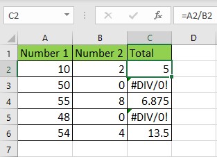
1. Handling Division by Zero

In many Excel models, dividing by zero leads to the #DIV/0! error. Instead of leaving this error visible in your worksheet, you can use IFERROR to manage it.

Example:

=IFERROR(E2/F2,"Error:Division by zero")


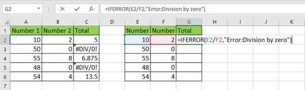
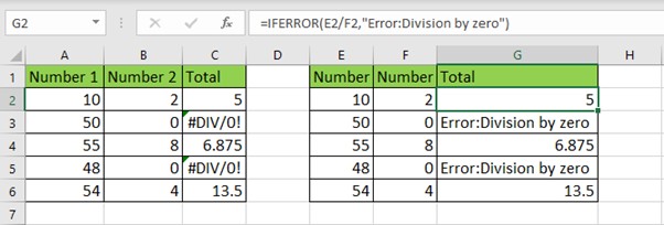
If F2 contains zero, the formula will return "Error: Division by zero" instead of the #DIV/0! message.

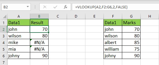
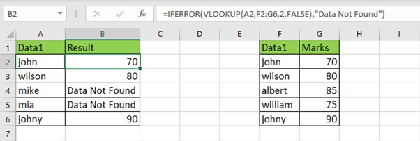
2. Cleansing Data from External Sources

When you import data from external systems, you might encounter incomplete data, leading to errors. IFERROR can help by cleaning up the output and providing more readable results.

Example:

=IFERROR(VLOOKUP(A2,F2:G6,2,FALSE),"Data Not Found")


If the VLOOKUP cannot find a match, IFERROR will return "Data not found" instead of the #N/A error.

3. Error Handling in Complex Calculations

If you’re using complex formulas that reference multiple sheets or datasets, an error at any point can break the entire calculation. IFERROR provides a safeguard for such scenarios.

Example:

=IFERROR(SUM(A1:A10)/SUM(B1:B10), "Calculation Error")

This formula will return "Calculation Error" if SUM(B1:B10) equals zero, preventing the #DIV/0! error.

Why Use IFERROR?

1. Improves Data Presentation: Replacing errors with meaningful messages makes your data easier to understand.

2. Boosts Productivity: Instead of manually checking and fixing errors, IFERROR automates the process.

3. Prevents Broken Formulas: In models that use multiple functions and references, IFERROR ensures that a single error doesn't disrupt the entire calculation.

IFERROR vs. IF Function: What’s the Difference?

You may wonder if you can handle errors with a simple IF function. While it’s true that IF can be used to manage certain errors, it’s not as efficient as IFERROR. With IF, you need to manually set up conditions for each possible error, which can become cumbersome. On the other hand, IFERROR automatically catches any error and handles it in one step, making it a more streamlined solution.

Conclusion

The IFERROR function is an essential tool for anyone working with formulas in Excel. It not only cleans up your data but also ensures that errors don’t disrupt your analysis. Whether you’re handling division by zero, incomplete data, or complex calculations, IFERROR can save you time and headaches.


Comments

Popular

FILTER Function in Excel with Example

Excel is a powerful tool with a myriad of functions that can simplify data management and analysis. Among its extensive repertoire, the FILTER function stands out for its ability to dynamically extract data based on specific criteria. While it may not be as widely known as functions like VLOOKUP or SUMIF, FILTER can be a game-changer when it comes to handling complex data sets.  In this blog post, we’ll dive deep into the FILTER function, exploring its syntax, use cases, and practical examples. By the end, you’ll be able to harness this function to make your data analysis more efficient and dynamic. What is the FILTER Function? The FILTER function is a part of Excel’s suite of dynamic array functions, introduced in Excel 365 and Excel 2019. It allows you to extract a range of data that meets specific criteria, automatically adjusting as the data changes. This makes it a powerful tool for creating custom views of your data without the need for complex formulas or manual adjustm...

HLOOKUP Function in Excel with Example

If you've ever worked with horizontal datasets in Excel and needed to find a specific value, the HLOOKUP function is your go-to tool. Short for "Horizontal Lookup," HLOOKUP allows you to search for a value across the top row of a table and return information from a specified row below. It’s particularly useful when managing spreadsheets with data organized in a horizontal format. In this post, we'll dive into how HLOOKUP works, why it’s useful, and how to apply it in various scenarios. What is HLOOKUP? The HLOOKUP function searches for a specific value in the top row of a table and returns data from a row you specify. It’s like the vertical counterpart, VLOOKUP, but designed for datasets where values are arranged horizontally. HLOOKUP Syntax: =HLOOKUP(lookup_value, table_array, row_index_num, [range_lookup]) lookup_value : The value you want to find in the first row. table_array : The range of data you want to search in. row_index_num : The ...

SWITCH Function in Excel with Example

In the world of Excel formulas, versatility and efficiency are key. One such tool that enhances both is the SWITCH function, which allows you to test an expression against multiple conditions and return the corresponding result. This function is often used in place of multiple IF statements, making your formulas more readable and easier to manage. What is the SWITCH Function? The SWITCH function in Excel evaluates an expression against a list of possible values and returns a corresponding result based on the first matching value. If no match is found, it can return a default result. This function is particularly useful for simplifying complex IF statements that involve several comparisons. Syntax of SWITCH Function The syntax for the SWITCH function is as follows: =SWITCH(expression, value1, result1, [value2, result2], ..., [default]) Expression : The value or cell that you want to evaluate. Value1, Value2, ... : The values you want to compare against the e...

How to Remove Virus from Removable Disk

Introduction Are you wondering how to remove a virus from a removable disk like a USB drive, external hard drive, or SD card? Removable disks can easily become infected with viruses that corrupt files, create shortcuts, or hide valuable data. In this SEO-optimized guide, we’ll show you how to remove viruses from your removable disk in simple steps, helping you keep your files safe, and your devices secure. Why Do Removable Disks Get Viruses? Viruses spread to removable disks when they’re connected to infected computers or used in public or shared computers. Understanding how viruses spread and how they affect your removable disk is essential for keeping your data safe. This guide will cover the most common signs of a virus on a USB drive and step-by-step instructions to remove viruses from removable disks . Signs Your Removable Disk May Be Infected with a Virus Before you start virus removal, here are some common signs your removable disk is infected: Unusual Files – Ne...

IFS Function in Excel with Example

In the world of Excel, performing logical tests is an essential skill that helps users analyse data, make decisions, and solve problems efficiently. One of the most powerful functions in Excel for this purpose is the IFS function. While many are familiar with the basic IF function, the IFS function takes conditional testing to the next level by allowing you to test multiple conditions at once, without needing to nest multiple IF statements. In this post, we will explain the working of the Excel IFS function, its usage, advantages, and provide practical examples to showcase how this function can simplify your workflow. What is the IFS Function? The IFS function in Excel is a logical function introduced in Excel 2016 that simplifies complex conditional tests. It evaluates multiple conditions in the order specified and returns a value corresponding to the first TRUE condition. If none of the conditions are met, an error will be returned unless a default condition is provided. The ...

IF function in excel with Example

The Excel IF formula is one of the most frequently used functions in spreadsheet operations. Its power lies in its ability to create logical comparisons between a value and what you expect. The function allows Excel users to automate tasks, analyse data more efficiently, and manage large datasets without manually reviewing every entry. In this detailed guide, you’ll learn how to harness the full potential of the IF formula, and we’ll dive deep into its variations and best practices. What is the IF Formula? At its core, the Excel IF formula performs a logical test, and based on the outcome of that test, it returns one of two results. It’s a basic yet versatile function that can handle a wide range of applications in financial modelling, data analysis, inventory management, and even project planning. Here’s the syntax for the IF formula: =IF(logical_test, value_if_true, value_if_false) In this syntax: 1.   logical_test : This is the condition or criteria that you want to ...

VLOOKUP Formula in Excel with Example

VLOOKUP (Vertical Lookup) is one of Excel’s most powerful and widely used functions. It allows users to search for a value in the first column of a range and return a corresponding value in the same row from another column. Whether you are managing inventory, financial data, or customer information, VLOOKUP helps save time by automating data retrieval across large datasets. How VLOOKUP Works VLOOKUP scans the column of a given range for a specific value, then returns the corresponding data from a different column. Here’s the basic structure of the VLOOKUP formula: =VLOOKUP(lookup_value, table_array, col_index_num, [range_lookup]) lookup_value : The value you want to find in the first column of the table. table_array : The range that contains the data (columns from which the function will pull). col_index_num : The column number from which you want to retrieve the value. [range_lookup] : Optional parameter (TRUE for approximate matches, FALSE for ex...

Excel SUMIF Function Explained with Real Examples

If you work with numbers in Excel, there's one function you must master: SUMIF. It’s simple, powerful, and one of the most searched formulas globally. Whether you’re managing sales data, budgets, or reports, SUMIF helps you add values based on conditions — no filters needed. WHAT IS THE SUMIF FUNCTION? The SUMIF function adds numbers in a range only if they meet a given condition. Syntax: =SUMIF(range, criteria, [sum_range]) - range – The cells to test against your condition- criteria – The condition to match - sum_range (optional) – The cells to actually sum (if different from range) Example 1: Add Sales Greater Than 100 Example Data: Product Sales A 120 B 80 C 150 If you need the sum of product whose sales more than 100 then the formula will be: =SUMIF(A2:B4,">100") Result: 270 (120 + 150) Example 2: Sum Based on Text Match Example Data: Product Sales ...